How to pull data from another sheet in Excel

Excel is a data management tool that has been frequently preferred by both individuals and businesses for many years. It is frequently preferred for many data management operations, from simple spreadsheets to more complex data clusters. Excel pull data from another sheet feature is one of the commonly preferred features by Excel users. Pulling data from another sheet in Excel allows users to easily get data from different worksheets and combine this data in a single location for simpler data analysis. Although Excel pull data from another sheet feature seems easy for many users, it actually contains many complicated steps and you should make sure that you thoroughly understand how to pull data from another sheet in Excel in order to avoid making mistakes. Let's see how to pull data from another sheet in Excel together!

Table of contents

• Fundamentals of referencing in Excel
• INDEX function to retrieve information from another Excel worksheet
• VLOOKUP function to retrieve data from another Excel worksheet
• MATCH function to find data in another Excel worksheet
• SUMIFS function to retrieving data from multiple Excel worksheets
• INDIRECT function to reference a worksheet name in a formula
• Combining data from multiple Excel worksheets into one with consolidation
• Common issues when pulling information from Aanother Excel worksheet
• Best practices for pulling data across multiple sheets in Excel
• Easiest way to pull data from another worksheets

Fundamentals of referencing in Excel

There are various methods to pull data from another sheet in Excel. Before we dive deeper into all these methods, let's start by understanding the basics of referencing in Excel.

Referencing between worksheets or workbooks in Excel is a way to define a cell or range of cells in any table. References always point to a specific cell or range of cells, so even if the data within those cells changes, the references are not affected.

It is very simple to refer to cells in the same worksheet. For example, to reference cell C8, you can type =C8 in another cell. However, referencing cells in a different worksheet is more complicated. You must also include the page name.

When referencing cells in a different workbook, you should not forget to add both the name of the worksheet and the name of the workbook. This method is called the external reference. It is a method you can use when you need to pull data from more than one workbook into a single worksheet or when you want to link data. If you're curious about how to link Excel sheets there are several methods you can use for this depending on your needs. Let's check the most popular methods for pulling data from another sheet in Excel!

INDEX function to retrieve information from another Excel worksheet

The INDEX function is used to return a specific value from a table or range of cells. The INDEX function is useful for pulling data from another sheet in an Excel workbook.‍

The syntax for the INDEX function is;

‍=INDEX(array,row_num,column_num)

• ‍Array: The array argument is the range of cells you want to pull the data from. ‍
• The row_num: The row_num arguments indicate the position of the data you want to pull within the array.‍
• The column_num: The column_num arguments indicate the position of the data you want to pull within the array.

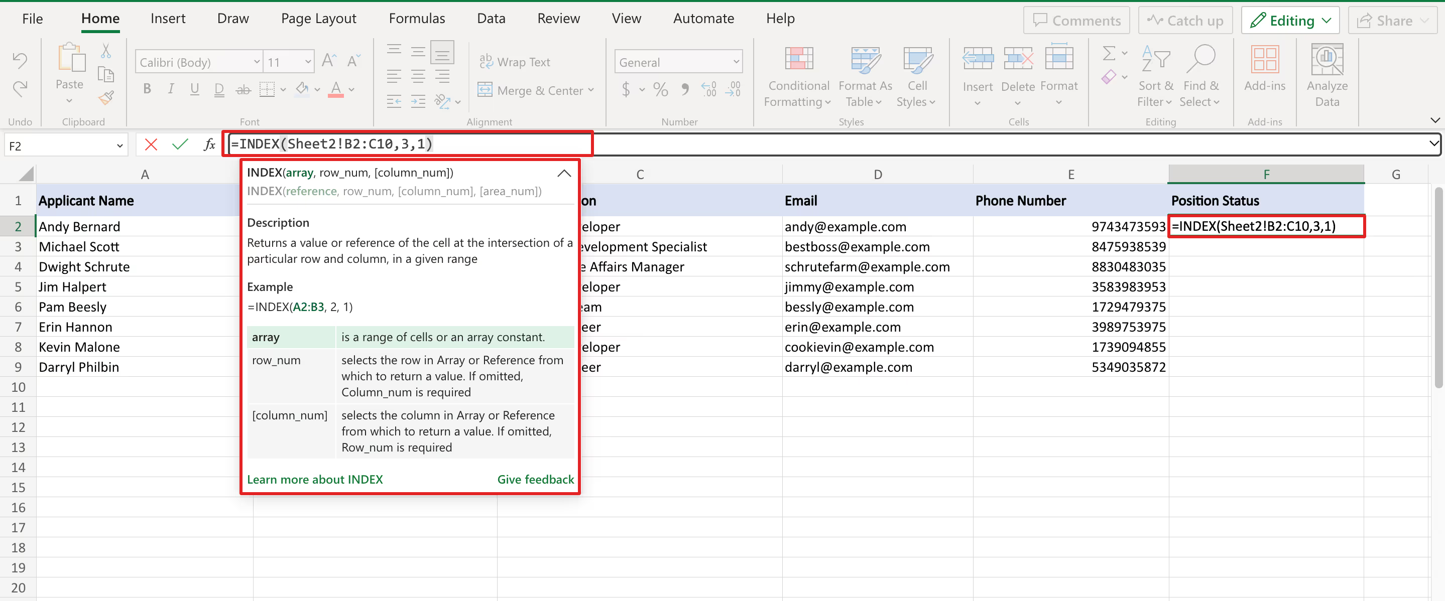
Note that you need to add the worksheet name in the array argument to use the INDEX function to pull data from another sheet.
For example, if you want to pull data from Sheet2 in a workbook, the syntax would be =INDEX(Sheet2!C2:B10,3,1). This will return the value in the third row and first column of the range C2:B10 in Sheet 8.

The INDEX function can also be combined with other Excel functions, such as MATCH and IF, to create more complex formulas.

You can use the MATCH function to find the position of a specific value in a range and then use the INDEX function to pull the corresponding value from another worksheet. This can be helpful when working with big datasets or when you need to do calculations based on data from multiple worksheets.

VLOOKUP function to retrieve data from another Excel worksheet

The VLOOKUP function is one of the most used functions for pulling data from another sheet in an Excel workbook. The VLOOKUP function allows you to search for a specific value in a table and return a corresponding value from a specified column.

The syntax for the VLOOKUP function is;

=VLOOKUP(lookup_value,table_array,col_index_num,range_lookup)

• The lookup_value: The lookup_value is the value you want to search.
• The table_array: The table_array is the range of cells that contains the table.
• The col_index_num: The col_index_num is the column number that contains the value you want to retrieve.
• The range_lookup: The range_lookup argument indicates whether you want to find an exact match or an approximate match.

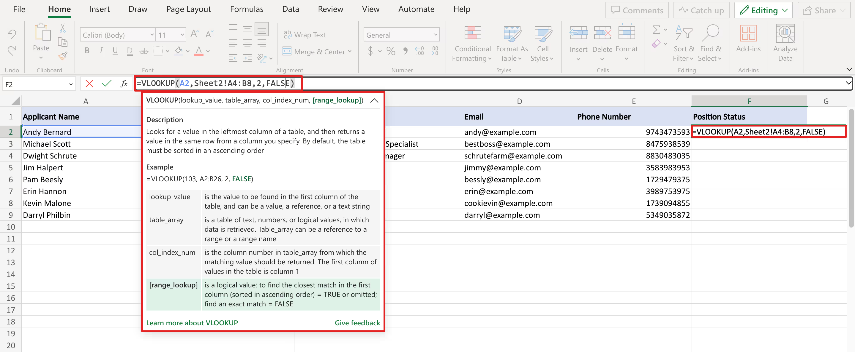
To use the VLOOKUP function to pull data from another Excel worksheet, you will need to include the worksheet name in the table_array argument. For example, if you want to retrieve data from Sheet2 in a workbook, the syntax would be =VLOOKUP(A2,Sheet2!A4:B8,2,FALSE). This will search for the value in cell A2 in the range A4:B8 in Sheet 8 and return the corresponding value from the second column.

MATCH function to find data in another Excel worksheet

The MATCH function allows you to search for a specific value in a range of cells and return its position within the range.

The syntax for the MATCH function is;
=MATCH(lookup_value,lookup_array,match_type)

• The lookup_value: The lookup_value is the value you want to search for.
• The lookup_array: The lookup_array is the range of cells you want to search.
• The match_type: The match_type argument indicates whether you want to find an exact match or an approximate match.

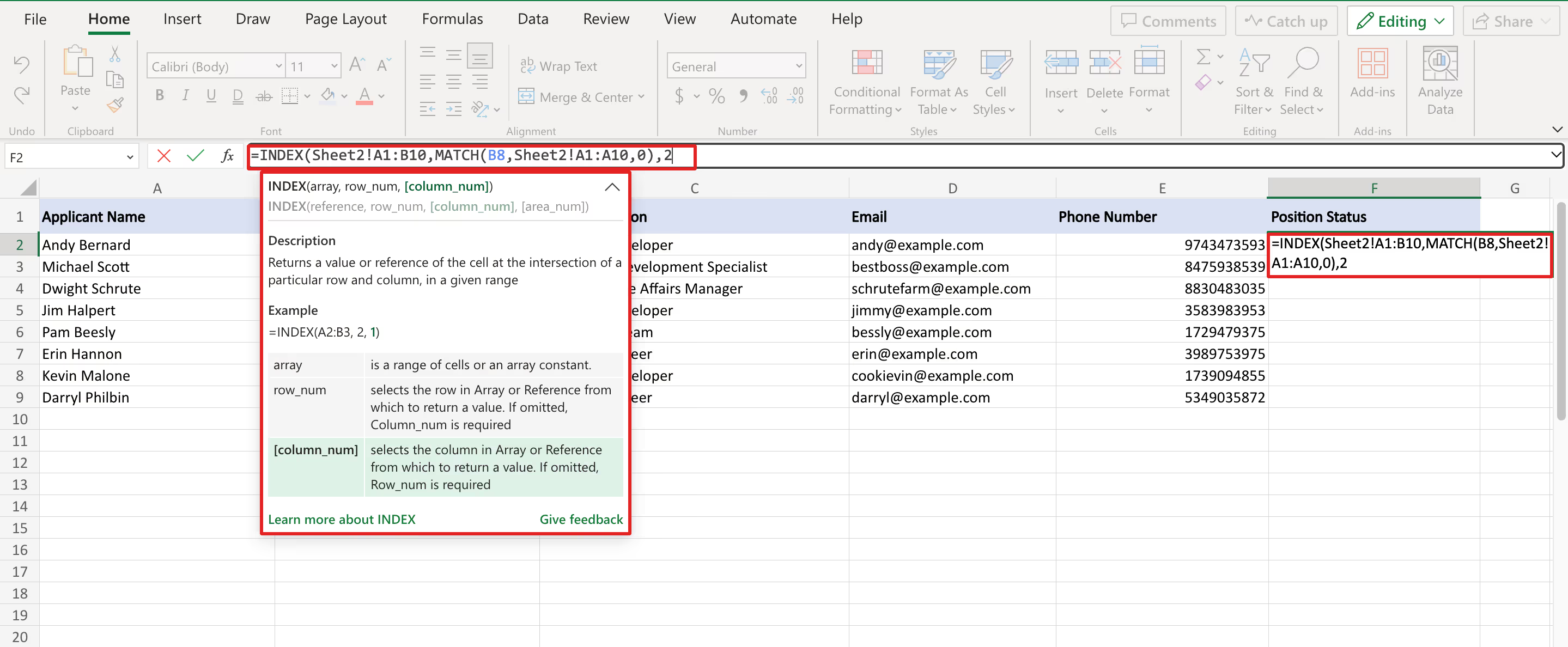
The MATCH function can pull data from another Excel worksheet when used with the INDEX function. For example, if you want to pull the value in cell B8 from Sheet2 in a workbook, you can use the following formula: =INDEX(Sheet2!A1:B10,MATCH(B8,Sheet2!A1:A10,0),2). This will search for the value in cell B8 in the range A1:A10 in Sheet2 and return the corresponding value from the second column of the range A1:B10 in Sheet2.

SUMIFS function to retrieving data from multiple Excel worksheets

The SUMIFS function is another helpful function for pulling data from multiple Excel worksheets in an Excel workbook. The SUMIFS function allows you to sum values from different Excel worksheets based on multiple criteria.
The syntax for the SUMIFS function is;

=SUMIFS(sum_range,criteria_range1,criteria1,criteria_range2,criteria2,....).

• The sum_range: The sum_range is the range of cells you want to sum.
• The criteria_range: The criteria_range specifies the sum conditions.
• The criteria: The criteria arguments specify the sum conditions.

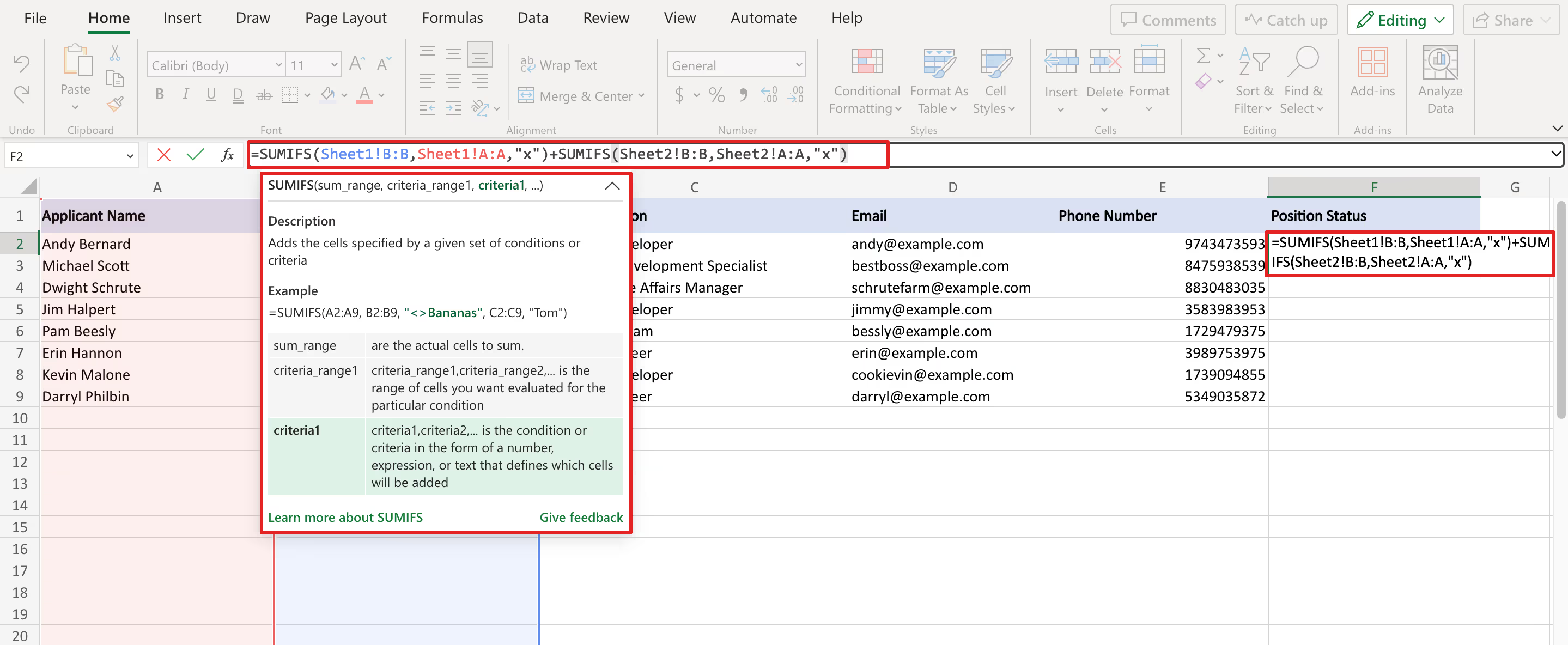
For example, if you have data in Sheet1 and Sheet2 and want to sum the values in column B in both sheets where the values in column A are equal to "x", you can use the following formula: =SUMIFS(Sheet1!B:B,Sheet1!A:A,"x")+SUMIFS(Sheet2!B:B,Sheet2!A:A,"x"). This will sum the values in column B in both worksheets where the value in column A equals "x".

INDIRECT function to reference a worksheet name in a formula

The INDIRECT function is one of the key functions for referencing data from other sheets in Excel. It allows you to create a reference to a cell or range of cells by constructing a text string that includes a reference to the worksheet name.
The syntax for the INDIRECT function is;
=INDIRECT(ref_text, [a1]).

• ‍‍The ref_text: The ref_text argument is the text string that contains the reference
• a1: The optional a1 argument indicates whether the reference is in A1 or R1C1 style.

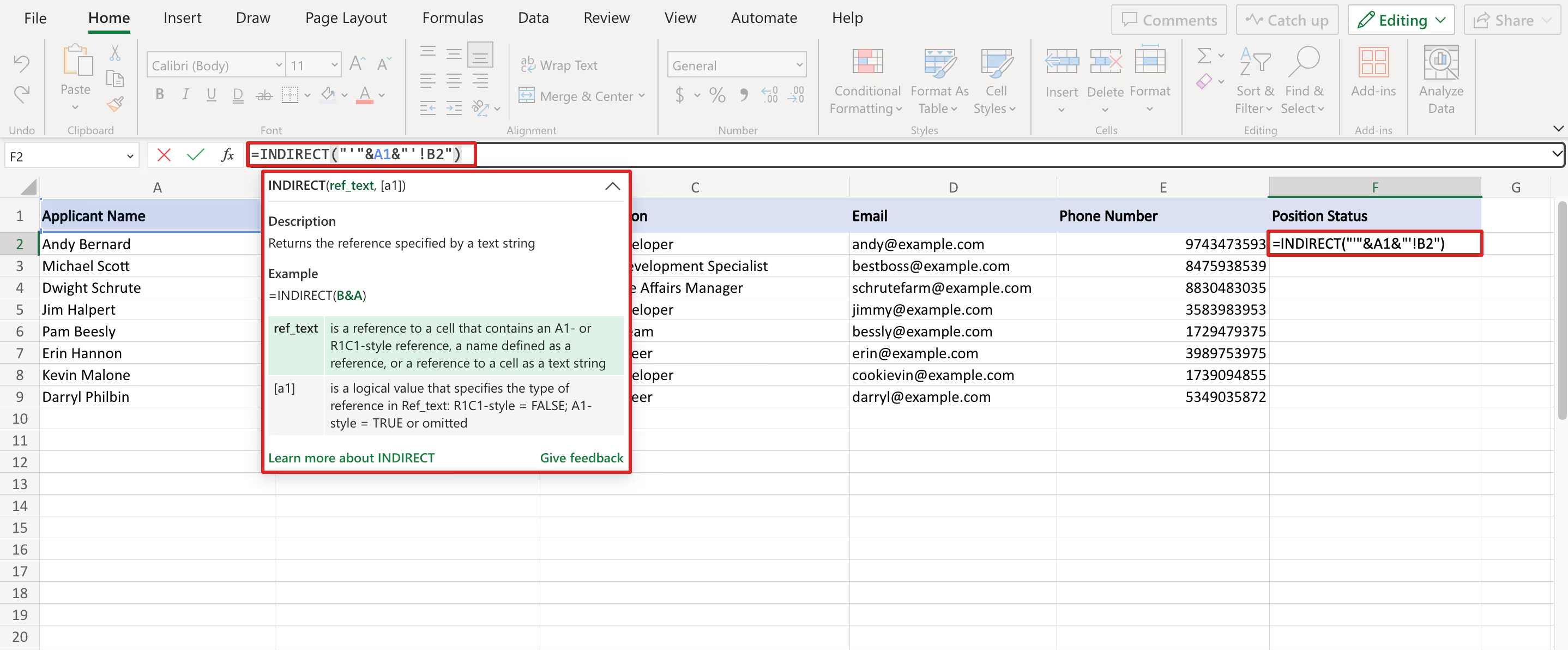
For example, if you have a drop-down list in cell A1 of Sheet4 that contains the names of different worksheets in the workbook, and you want to pull the value in cell B2 of the selected sheet, you can use the following formula: =INDIRECT("'"&A1&"'!B2"). This will create a reference to the cell B2 of the selected sheet and return its value.

Combining data from multiple Excel worksheets into one with consolidation

The consolidation feature of Excel allows you to combine data from multiple worksheets into one. The consolidation feature can be useful when you have a big dataset spread across multiple Excel worksheets or workbooks. You can select the "Consolidate" option in the "Data" menu to use the consolidation feature.

Then, you can select the range of cells you want to consolidate and choose the function you want to use (SUM, COUNT, AVERAGE, etc.). So, Excel will create a new worksheet that contains the consolidated data.

Common issues when pulling information from another Excel worksheet

If the question "How to pull data from another sheet in Excel" constantly bothers you and you constantly experience problems related to it, you can detect your mistakes by paying attention to these common issues. While pulling data from another Excel worksheet, you may have some common issues.

One of the most common issues is #REF! errors. It occurs when the reference you're using is not valid. To fix the #REF! issue, you should make sure you're using the correct worksheet name and that the cells and ranges you're referencing exist in the worksheet.

Another common issue is circular references, it occurs when a formula refers back to itself. To fix the issue of the circular reference, you can adjust the formula to remove the circular reference or enable iterative calculations in Excel.

Best practices for pulling data across multiple sheets in Excel

If you think you understand How to pull data from another sheet in Excel well enough, you should make sure that you comply with some best practices. When pulling data across multiple worksheets in Excel, it's crucial to follow some best practices to avoid common errors and improve the performance of your data operations.
‍

Using named ranges instead of cell references is one of the best practices and it is easier to manage and less prone to errors.

Another best practice is to use relative references whenever possible while pulling data from another sheet in Excel. This reduces the risk of errors when moving or copying formulas between worksheets. Also, it's essential to check your formulas for errors regularly and to ensure that any changes you make to the data or structure of the workbook don't break your Excel formulas.

With these common best practices, you can ensure that your Excel formulas work properly and that you can easily pull data from other worksheets in Excel

Easiest way to pull data from another worksheets

Many users have difficulty finding the answer to the question of how to pull data from another sheet in Excel. Because Excel has various formulations that allow you to pull data from different worksheets and workbooks. If you are an expert in Excel, these methods may be functional for you. However, as we mentioned in our article, Excel's functions that help you pull data from different worksheets and workbooks are very sensitive and it is very easy for these formulas to be corrupted by any mistake, especially in spreadsheets on which you work together with your teammates. For critical data management operations, this can be quite sensitive and risky. At the same time, if you are not an expert in Excel, such complex operations may increase your manual workload and cause you to lose time.

New-generation smart online spreadsheet tools have features that make it easier to pull data from different data tables. Thus, even if you are not an expert in Excel, you can easily exchange data between your tables and have spreadsheets containing references created quickly and easily. In addition, new-generation online spreadsheet tools are very effective for teams that collaborate on spreadsheets. This way, it won't be a problem for you if one of your teammates accidentally breaks a formula.

Let's check together how you can reference and pull data between different data tables using Retable!

• Open your Retable dashboard
• Create a project under one of your workspaces
• Create 2 tables on the same project
• Enter your data in the relevant tables and choose your column types
• Let's say you want to pull data from the 2nd worksheet to the 1st worksheet, for this go to your 1st worksheet.
• Go to the column you want to set as the reference.
• Set your column type as "Reference Another Table"
• Select the table and column to reference
• That's all, now your reference is ready.

Bonus: You can also bring the other data in the row of the cell in a table you refer to your table with one click via the "Look Up" column.

Let's see how it works!

• Create a "Look-up Values" column
• Select your "Referenced column"
• Select your "Lookup column"
• And save it! That's all!

Now your Look-up Values column is ready. You can automatically get the date from the referenced table and columns.

Try linking two worksheets in your own online spreadsheets! Easily get records from different worksheets and avoid incorrect data entry, create relational databases by easily creating connections between your data.